
Decision Trees, Neural Networks and the Machine-Learning Stack Behind MSME Credit Ratings
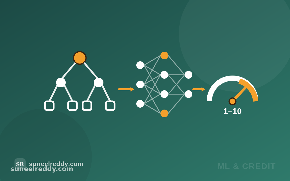
A technical walkthrough of the model stack behind modern MSME rating engines — what each algorithm contributes, the formulas that matter, and the unglamorous machinery (calibration, explainability, monitoring) that turns a prediction into a defensible credit decision. Illustrative frameworks, not lending advice.
An MSME credit rating is really three problems wearing one name: estimation (what is this borrower's probability of default?), calibration (how do I turn that probability into a stable 1–10 grade?), and decisioning (at what grade, price and limit do I say yes?). Machine learning has transformed the first problem, disciplined the second, and — if governed well — sharpened the third. Here is how the pieces fit.
The raw material: what an MSME model actually eats
For an Indian MSME, a modern feature set draws from four layers, in rough order of predictive power:
- Bureau layer. CMR/CIMR rank, months on book, enquiry velocity, worst-ever DPD, utilisation of existing limits, promoter's consumer score and its trend.
- Cash-flow layer. From bank statements via Account Aggregator: monthly credit turnover and its volatility, counterparty count, bounce rate, minimum-balance days, drawdown behaviour on CC limits.
- Compliance layer. GST filing regularity, GSTR-1 vs GSTR-3B consistency, turnover growth from invoice data, EPFO payment discipline.
- Firmographic layer. Sector, age, geography, Udyam class, customer-concentration proxies from invoice data.
A practical note that outweighs any algorithm choice: the label matters more than the model. Define default precisely (90+ DPD within 12 months of observation is common), fix the observation/performance window, and exclude fraud cases — fraud is a different model. Most “ML lifted our Gini by 8 points” stories are really “we cleaned our target variable” stories.
The baseline everyone must beat: the logistic scorecard
The industry workhorse is logistic regression on weight-of-evidence (WOE) transformed variables. Each feature is binned, and each bin i gets WOE(i) = ln(% of goods in bin ÷ % of bads in bin); the model is then log(p/(1−p)) = β0 + Σ βk·WOEk. Scores are scaled with the points-to-double-odds convention: Score = Offset + Factor × ln(odds), where Factor = PDO/ln(2) — so with PDO = 20, every 20 points doubles the odds of being good.
Why start here? The scorecard is monotonic by construction, every point movement has a stated reason, regulators have four decades of validation methodology for it, and it sets the Gini benchmark. On thin MSME datasets (a few thousand defaults), a well-binned scorecard is embarrassingly hard to beat.
Decision trees: the interpretable cut-finder
A CART tree recursively splits the portfolio on the feature and threshold that maximise impurity reduction — using Gini impurity, G = 1 − Σ pk², or entropy. For MSME credit, single trees earn their keep in three places: discovering interaction cut-points (e.g., “GST-filing gaps only predict default when banking volatility is also high”) that then feed the scorecard as engineered features; policy rule mining (converting a tree path into a transparent knockout rule); and segmentation — growing a shallow tree to split the portfolio into homogeneous sub-populations (trader vs. manufacturer vs. services), each getting its own scorecard.
Their weakness is instability: resample the data and the tree redraws itself. That is exactly what ensembles fix.
Ensembles: random forests and gradient boosting
Random forests average hundreds of decorrelated trees (bagging + random feature subsets). They are robust, nearly tuning-free, and a good second benchmark — but they plateau.
Gradient boosting (XGBoost, LightGBM, CatBoost) is the current state of the art on tabular credit data, and most modern MSME engines — including the standardised digital assessment models Indian PSBs have begun rolling out — are built on this family. Boosting fits trees sequentially, each one on the gradient of the loss left by the last, minimising a regularised objective: L = Σ l(yi, ŷi) + Σ [γT + ½λ‖w‖²] — the γT term penalising tree size, λ the leaf weights. In published SME studies, boosted models beat logistic baselines on AUC, precision and recall, especially when paired with SMOTE or class-weighting to handle the 30:1 good-to-bad imbalance typical of credit data.
Practitioner defaults that save grief: cap tree depth at 3–5 (credit signals are shallow-interaction), use early stopping on a time-out-of-sample fold — never a random fold, because credit data drifts — and enforce monotonicity constraints (higher utilisation must never lower predicted risk), which modern GBM libraries support natively and which regulators increasingly expect.
Neural networks: where they earn their place, and where they don't
On flat tabular features, a multi-layer perceptron rarely beats tuned gradient boosting — published comparisons repeatedly land there, and the deep-learning literature concedes tabular data to trees. Neural networks justify their governance cost in MSME credit in three specific roles:
- Sequence models over transactions. An LSTM or small transformer reading 24 months of raw bank-statement flows (daily balances, credit/debit rhythms) learns liquidity-stress signatures that hand-engineered monthly aggregates blur away. This is the highest-value NN application for cash-flow lending.
- Entity embeddings. Learned dense representations of high-cardinality categoricals — pincode, industry code, anchor buyer — that feed back into a GBM as features.
- Hybrid stacks. NN-derived features + GBM head, or an ensemble average of scorecard + GBM + NN. Diversity buys 1–2 Gini points at the top of the leaderboard.
The trade: NNs need more data than most MSME books have, are harder to explain, and drift silently. If your default count is under ~5,000, spend the effort on features, not architecture.
From probability to rating: calibration and the master scale
A model outputs a score; a rating system needs a calibrated PD. Two steps:
First, map scores to true probabilities with Platt scaling (a logistic fit on the validation set) or isotonic regression; verify with a calibration plot and Brier score. Boosted models are usually miscalibrated out of the box — confident at the extremes — and this step is not optional when PD feeds pricing or ECL provisioning.
Second, band PDs into grades on a master scale, mirroring how CMR or an internal 1–10 scale works:
| Grade | PD band | Indicative decision |
|---|---|---|
| 1–2 | < 0.5% | Auto-approve, finest pricing |
| 3–4 | 0.5–2% | Approve, standard pricing |
| 5–6 | 2–5% | Approve with structure/collateral |
| 7–8 | 5–12% | Manual review, price for risk |
| 9–10 | > 12% | Decline or secured-only |
Grade boundaries should be set so grades are stable (borrowers don't oscillate monthly), monotonic in observed default rates (validated annually), and meaningfully populated — a grade nobody occupies is a grade that teaches you nothing.
Explainability: SHAP, reason codes, and the regulator
Every declined MSME deserves — and in most regimes is owed — a reason. SHAP (Shapley additive explanations) decomposes any prediction into per-feature contributions: f(x) = φ0 + Σ φi, with TreeSHAP computing this exactly and fast for tree ensembles. In practice: global SHAP summaries for model governance (what drives the book), local SHAP values for adverse-action reason codes (top negative contributors, translated into plain language), and SHAP-interaction scans to catch proxy discrimination — a pincode variable quietly encoding what regulation forbids you to use directly.
Governance is now the binding constraint, not accuracy. Basel-style model risk management — independent validation, documentation, challenger models, human override rights — applies with extra force to ML models whose validation methodology is still maturing. The pragmatic pattern most lenders adopt: a scorecard as the model of record, a GBM as challenger, promoted only when it beats the incumbent out-of-time for several consecutive quarters, with SHAP wired into every decision it touches.
Monitoring: the model after the model
A rating engine is a depreciating asset. The maintenance schedule:
- Discrimination: AUC/Gini and KS on rolling out-of-time cohorts; investigate any sustained Gini decay >5 points.
- Stability: Population Stability Index, PSI = Σ (Ai − Ei)·ln(Ai/Ei) per feature and on the score itself; PSI > 0.25 means the through-the-door population no longer resembles training data — common after a GST rule change or a new sourcing channel.
- Calibration: realised vs. predicted default rate per grade, with binomial tests; recalibrate annually, rebuild when drift is structural.
- Vintage analysis: cumulative default curves by origination quarter — the earliest honest verdict on whether the model (and the cutoff) is working.
The decision layer: where the money actually is
The cutoff, not the model, determines profit. For each score band, expected profit ≈ (1−PD)·margin − PD·LGD·EAD; approve where it's positive, and test cutoff moves with swap-set analysis — who do we newly approve, who do we newly decline, and what were their actual outcomes? Layer on champion/challenger decisioning (route a small random slice past the cutoff to keep learning about rejected populations — otherwise reject inference calcifies your bias), and let the grade drive structure, not just yes/no: grade 5–6 borrowers get anchor-backed TReDS lines or CGTMSE cover rather than clean limits.
The honest summary
Decision trees find the cut-points, boosting squeezes the signal, neural networks read the raw cash-flow tape, and the logistic scorecard keeps everyone honest. But the durable edge in MSME rating isn't the algorithm — algorithms are public. It's the label discipline, the calibration, the monitoring cadence, and the courage to keep a human override where the data is thin. The model computes the rating; the system around it earns the right to use it.
References
Beneish/Altman lineage aside — for this stack: Chen & Guestrin (2016), “XGBoost: A Scalable Tree Boosting System.” Lundberg & Lee (2017), “A Unified Approach to Interpreting Model Predictions” (SHAP); TreeSHAP (2020). Siddiqi, N. — “Credit Risk Scorecards” (WOE/PDO methodology). Breiman et al. — CART (1984); Breiman (2001), “Random Forests.” Chawla et al. (2002) — SMOTE. Published SME/MSME ML comparisons: PMC — “Credit risk assessment of small and micro enterprise based on machine learning”; arXiv — ensemble + SHAP credit default studies; Nature Sci. Reports — explainable hybrid credit models. KNN India — PSB standardised digital MSME credit assessment rollout. Basel Committee / RBI — model risk management and validation expectations.